User Manual

IonGAP has been designed with the aim of simplifying your work, and our Web interface has a lot to do with it. Creating a project in IonGAP is so simple as following the next steps:

Click here or use the Home tab of the navigation bar to go to the Home page. Then, click the Start New Project button under the platform description.

In the New Project form, you will see four sections:

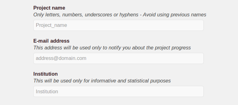
1. A first section where you must fill a few mandatory fields:
   • Project name: a descriptive identifier for the project (usually, the organism name). It must be 3 to 50 characters long, containing only letters, numbers, underscores or hyphens. It is advisable to avoid using previous project names.
   • Email address: this address will be used exclusively to notify you once the project has started, as well as once it is complete. It will not be used in any other way, nor transferred to anyone external to the service.
   • Institution: the name of the institution you belong to will be used only with informative/statistical purposes. It must contain only letters, numbers, spaces, underscores or hyphens.

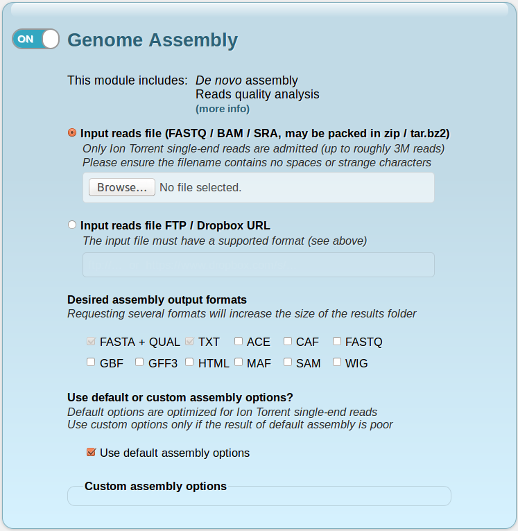
2. A blue section corresponding to the Genome Assembly module of the service, which you can enable or disable by clicking on the switch in the upper left corner. When enabled, it contains the following fields:
   • Input reads file: this is the only file needed to perform the assembly. It must have FASTQ (.fastq, .fq), BAM (.bam) or SRA (.sra) format, and its name cannot contain spaces or strange characters (such as slashes, asterisks, brackets or parentheses). IonGAP allows compressed files in zip or tar.bz2 format, which can be obtained directly from the Torrent Server's FileExporter plugin and are useful in order to reduce the upload time. Currently, IonGAP admits datasets of up to roughly 3 million Ion Torrent single-end reads. This corresponds to about 1 GB in FASTQ format (the size will vary largely depending on the input format). You can attach the file by clicking the Browse... button.
   • Input reads file FTP / Dropbox URL: alternatively, you can supply a FTP or a shared Dropbox URL to your reads file (which must be in one of the admitted formats, see above). This helps to avoid long upload times, especially when using the same file in several projects. Please ensure that the URL follows the form indicated in this text field.
   • Desired assembly output formats: here you can choose between 9 optional output file formats for the assembly module. The default formats are FASTA + QUAL and TXT.
   • Use default assembly options: by unchecking this option, you can specify a custom assembly configuration, changing any of the 14 configurable assembly parameters. However, this is not advisable unless you are obtaining poor results using the default assembly configuration. The default parameter values come from an exhaustive comparative study on Ion Torrent single-end sequence data.

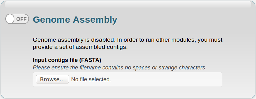
If you disable this module, a new panel will appear below, where you can submit a file containing your own assembled contigs. This file must be in FASTA (.fasta, .fna, .fas) format, and its name cannot contain spaces or strange characters (such as slashes, asterisks, brackets or parentheses).

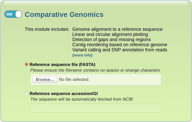
3. A green section regarding to the Comparative Genomics module, which you can enable or disable by clicking on the switch in the upper left corner. It contains the following fields:
• Reference sequence file: in order to perform the comparative analysis routines, you must provide a reference sequence file. This file must be in FASTA (.fasta, .fna, .fas) format, and its name cannot contain spaces or strange characters (such as slashes, asterisks, brackets or parentheses).
• Reference sequence accesion/GI: if your reference sequence is in the NCBI database, you don't need to download it. Simply type its accesion or GI number here, and IonGAP will take care of the rest.

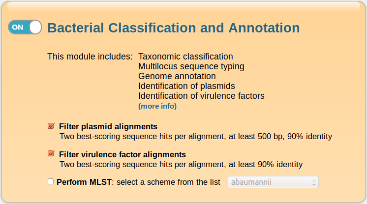
4. An orange section corresponding to the Bacterial Classification and Annotation module of the service, which you can enable or disable by clicking on the switch in the upper left corner. It contains the following fields:
• Filter plasmid alignments: uncheck this option if you want to get the unfiltered output of the identification of plasmids. If checked, only the two best-scoring plasmid sequence hits for each alignment, having at least 500-bp length and 90% identity, will be included.
• Filter virulence factor alignments: uncheck this option if you want to get the unfiltered output of the identification of virulence factors. If checked, only the two best-scoring sequence hits for each alignment, having at least 90% identity, will be included.
• Perform MLST: check this option if you want MLST to be performed and you know the organism species (scheme). If checked, you must select the scheme from the pull-down list.

Once you have filled the form, click the Start project button. A green label will appear, telling you to wait while your files are transferred. This process can take from 5 minutes to an hour, depending on the data size and the quality of your connection. You can use your computer normally meanwhile.

After the files have been uploaded, you will see a new page informing that your project has been started. You will receive an email notification to the address you provided when your project starts, as well as another email once it is complete, through which you will be able to download the project results.

Your project may be successful or fail. Failures occur during the assembly process, and they may be due to problems in the data file, an incorrect assembly configuration (if you defined custom assembly options), an excessive amount of data for the system, or an unexpected system failure.

Whether the assembly was successful or not, you will receive an informative email (check your spam folder otherwise) which includes a link for downloading the compressed project results file. If the project failed, this file will only contain the assembly process log, as well as a quality analysis of the reads file. If the project was successfully finished, you will find the structure of directories and files detailed below.

1. Assembly: contains the results of the assembly process (assembled contigs).
• Info: Contains informative files about the assembly.
• Name_AssemblyLog.txt: log of the whole assembly process.
• Name_ContigReads.tsv: information about the reads contained in each contig.
• Name_ContigStats.tsv: statistics about the contigs.
• Name_InfoAssembly.txt: basic information about the assembly. IonGAP outputs only the “large contigs” generated by MIRA.
• Name_LargeContigsList.txt: list of “large contigs”, which are the output of IonGAP.
• Name_ReadRepeats.tsv: information about which parts of which reads are repetitive in the project.
• Contigs: “large” contigs assembled by MIRA, in the formats specified by the user. The minimum length of “large” contigs can be set when starting the project, in the custom assembly options section.
• ACE: old assembly file format used mainly by phrap and consed. If you do not have consed, you might want to try clview to look at .ace files.
• BAM: the binary cousin of the SAM format.
• CAF: Common Assembly Format, developed by the Sanger Centre.
• FASTA: a simple format for sequence data. The padded version includes gaps (asterisks) in the consensus sequence; it can be visualized along with the SAM file in programs like Tablet, in order to explore the aligned assembly results (pileup of reads).
• FASTA.QUAL: an extension of FASTA format, used to also store quality values in a similar fashion.
• GBF: GenBank file format as used at the NCBI to describe sequences.
• GFF3: General Feature Format, used to describe sequences and features on these sequences.
• HTML: Hypertext Markup Language. Projects written in HTML format can be viewed directly with any Web browser.
• MAF: MIRA Assembly Format (MAF). A faster and more compact form than CAF or ACE, but it can only be read by MIRA.
• SAM: Sequence Alignment/Map Format.
• TXT: a human readable format for the aligned assembly results, where all input sequences are shown in the context of the contig they were assembled into. It is just meant as a quick way for people to have a look at their assembly without specialized alignment finishing tools.
• WIG: a genome coverage file format. It comes handy for searching genome deletions or duplications in programs like the Affymetrix Integrated Genome Browser, or when looking for foreign sequences in a genome.
• ReadsQuality: contains the reads quality report generated by FastQC.
• Name_ReadsQC.html: reads quality report in HTML format. This quality analysis has no impact on the project.
2. Bacterial: contains the results of the bacterial classification and annotation routines. If the Comparative Genomics module was enabled, these results are obtained from the reordered contigs set (Comparative/Reorder folder). The applications involved in each process are listed in the Tools and Features section.
• Annotation: contains the annotated contigs in different file formats.
• FAA: protein FASTA file of the translated CDS sequences.
• FFN: nucleotide FASTA file of all the annotated sequences, not just CDS.
• GBK: standard GenBank file derived from the master .gff.
• GFF: master annotation in GFF3 format, containing both sequences and annotations. It can be viewed directly in Artemis or IGV.
• SQN: an ASN1 format “Sequin” file for submission to GenBank. It needs to be edited to set the correct taxonomy, authors, related publication etc.
• TBL: feature Table file, used to create the .sqn file.
• TXT: statistics relating to the annotated features found.
• Classification: contains the result of the taxonomic classification of the contigs, based on 16S rRNA gene sequence alignments.
• Name_Classification.tsv: taxonomic classification table. For each matching contig, there are three raws in the table, corresponding to the best three alignments of the 16S ribosomal RNA gene, with at least 97% identity.
• MLST: contains the results of the multilocus sequence typing process.
• Name_Alleles.fasta: sequence of the ST alleles found in contigs.
• Name_MLST.tsv: MLST result table, containing the selected scheme (species), the MLST type (ST), and the allele variants for each of the locii within the scheme. Only full-length, 100% identity matches to an allelle are considered matches. If any allelles are not found, a “-” will be present in the allele column, as well as in the ST column.
• Plasmids: contains the results of the identification of plasmids.
• Name_Plasmids.tsv: table of NCBI annotated plasmids found within the “large contigs”. If the Comparative Genomics module was enabled, it could be distinguished between chromosomal integrated elements or plasmids (as extra-chromosomal elements). If the plasmids filter was selected when starting the project, only up to 2 hits per alignment site, with at least 500-bp length and 90% identity, are considered.
• Virulence: contains the results of the identification of virulence factors. If the virulence factors filter was selected when starting the project, only up to 2 hits per alignment site, with at least 90% identity, are considered.
• Name_AntibioticResistance.tsv: table of detected antibiotic resistance genes.
• Name_PathogenicityIslands.tsv: table of detected pathogenicity islands.
• Name_tRNAs.tsv: table of detected tRNAs (considered pathogenicity islands).
• Name_VirulenceProteins.tsv: table of detected virulence proteins, protein toxins, transcription factors and differential gene regulation elements (some categories may not be present).
3. Comparative: contains the results of the comparative genomics routines. The applications involved in each process are listed in the Tools and Features section.
• Alignment: contains the results of the alignment between the reordered contigs and the reference sequence.
• Name_Gaps.tsv: table of alignment gaps in both contigs and reference sequence.
• Name_MissingRegions.fasta: sequence of regions present in the reference but not in the assembly.
• Name_Summary.tsv: statistics about the alignment.
• AlignmentGraphs: contains different plots of the alignment between the original or reordered contigs and the reference sequence.
• Name_AlignmentLayout.png: transversal diagram of the alignment between the contigs and the reference sequence, where contigs are ordered and oriented in order to achieve the best possible alignment. The x-axis represents the position in the reference sequence, and the y- axis, the position in the different contigs (from bottom to top). The diagonal line shows the mapping of contigs to the reference sequence, where the red segments indicate that the depicted contigs are correctly oriented, while the blue ones represent contigs whose orientation is inverted with respect to the reference sequence.
• Name_AlignmentRaw.png: transversal diagram of the alignment between the original contigs and the reference sequence.
• Name_AlignmentView_Total.pdf: detailed linear alignment graph between the contigs and the reference sequence. The top blue bar represents the reference sequence, and the bold red bar, the coverage of the alignment. The best found alignment is depicted by the thin red line, which is accompanied by the name of each aligned contig. The x-axis represents the position in the reference sequence, and the y-axis, the percentage identity between both sequences. In case of large genomes, this graph may not be generated.
• Name_AlignmentView_1/2/3.pdf: This files contain the same alignment graph in Name_AlignmentView_Total.pdf, but splitted into 3 parts.
• Name_CircAlignment.pdf: circular diagram of the alignment between the reference sequence (left half) and the original contigs (right half). Matches are colored according to the percentage identity (from higher to lower: red, orange, green, blue), and have a fold in the middle if the contig is inverted with respect to the reference sequence. Only the 250 largest contigs are considered.
• Name_CircAlignment_Reorder.pdf: circular diagram of the alignment between the reference sequence (left half) and the reordered contigs (right half). Matches are colored according to the percentage identity (from higher to lower: red, orange, green, blue), and have a fold in the middle if the contig is inverted with respect to the reference sequence. Only the 250 largest contigs are considered.
• Name_CircCoverage.pdf: circular diagram of the coverage of the alignment between the reference sequence (left half) and the original contigs (right half). Only the 250 largest contigs are considered.
• Name_Coverage.png: linear diagram of the coverage of the alignment between the contigs and the reference sequence. The x-axis represents the position in the reference sequence, and the y-axis, the percentage identity of the mappings at that position. The red segments indicate that the depicted contigs are correctly oriented, while the blue ones represent contigs whose orientation is inverted with respect to the reference sequence. The lower line allows to visualize the portion of the reference sequence covered by the contigs.
• Name_LinearAlignment.pdf: linear diagram of the alignment between the contigs (above) and the reference sequence (below). Match ribbons are colored according to the percentage identity (the darker, the higher) and the contig orientation (blue if it is inverted with respect to the reference sequence, and red otherwise). The color of the alignments themselves (inside the contigs) is matched with the color of the corresponding segments in the reference sequence.
• Reorder: contains the reordered and reoriented contigs, using as a base the reference sequence.
• Name_ReorderedContigs.fasta: reordered and reoriented contigs, in FASTA format.
• Name_OriginalContigs.tsv: information about the position of the contigs in the original file.
• Name_ReorderedContigs.tsv: information about the final position and orientation of the reordered contigs.
• VariantCalling: contains the variant calls and annotated SNPs. These results are generated only if a set of reads was provided (i.e., if the Genome Assembly module was enabled).
• Name_SNPAnnotation.tsv: table of annotated SNPs, indicating their presumed effect on the genome, the most likely genotype according to the variant calling results (reference base or new base) and the genotype confidence (logarithm ratio between the most likely and the least likely genotype). If multiple SNPs occur in a single codon, all but the last one in that codon will be labelled “MNP” (Multiple Nucleotide Polymorphism). The annotation of the last SNP in the codon will then take the cumulative effect of all SNPs into account. Mutant types used to annotate SNPs and MNPs are synonymous (no change in amino acid), nonsynonymous (different amino acid), nonsense (normal codon replaced by stop codon), nonstop (stop codon replaced by normal codon) and nonstart (start codon at start of feature replaced by a normal codon).
• Name_VariantCalls.vcf: variant calls (SNPs, MNPs and indels) produced by Cortex, in VCF format.

In the main results directory you will also find an HTML file, named Name_Summary.html, which provides a summarized vision of the project results for each of the executed modules.

Windows users should use Word / WordPad instead of Notepad for reading text files. Tabular files (.tsv) can be opened with any spreadsheet application. To see output examples, please consult the Tools and Features section.